


El paquete de álgebra lineal de Tensorflow tiene una función, tf.linalg.svdque puede usarse para calcular la descomposición del valor singular de una o más matrices. Comience definiendo una matriz easy y calculando su factorización SVD.
A = tf.random.uniform(form=[40,30])
# Compute the SVD factorization
s, U, V = tf.linalg.svd(A)
# Outline Sigma and V Transpose
S = tf.linalg.diag(s)
V_T = tf.transpose(V)
# Reconstruct the unique matrix
A_svd = U@S@V_T
# Visualize
plt.bar(vary(len(s)), s);
plt.xlabel("Singular worth rank")
plt.ylabel("Singular worth")
plt.title("Bar graph of singular values");
WARNING: All log messages earlier than absl::InitializeLog() is known as are written to STDERR
I0000 00:00:1723689633.424919  126589 cuda_executor.cc:1015] profitable NUMA node learn from SysFS had unfavorable worth (-1), however there should be at the least one NUMA node, so returning NUMA node zero. See extra at
I0000 00:00:1723689633.428762  126589 cuda_executor.cc:1015] profitable NUMA node learn from SysFS had unfavorable worth (-1), however there should be at the least one NUMA node, so returning NUMA node zero. See extra at
I0000 00:00:1723689633.432420  126589 cuda_executor.cc:1015] profitable NUMA node learn from SysFS had unfavorable worth (-1), however there should be at the least one NUMA node, so returning NUMA node zero. See extra at
I0000 00:00:1723689633.437707  126589 cuda_executor.cc:1015] profitable NUMA node learn from SysFS had unfavorable worth (-1), however there should be at the least one NUMA node, so returning NUMA node zero. See extra at
I0000 00:00:1723689633.449819  126589 cuda_executor.cc:1015] profitable NUMA node learn from SysFS had unfavorable worth (-1), however there should be at the least one NUMA node, so returning NUMA node zero. See extra at
I0000 00:00:1723689633.453529  126589 cuda_executor.cc:1015] profitable NUMA node learn from SysFS had unfavorable worth (-1), however there should be at the least one NUMA node, so returning NUMA node zero. See extra at
I0000 00:00:1723689633.457079  126589 cuda_executor.cc:1015] profitable NUMA node learn from SysFS had unfavorable worth (-1), however there should be at the least one NUMA node, so returning NUMA node zero. See extra at
I0000 00:00:1723689633.460600  126589 cuda_executor.cc:1015] profitable NUMA node learn from SysFS had unfavorable worth (-1), however there should be at the least one NUMA node, so returning NUMA node zero. See extra at
I0000 00:00:1723689633.464019  126589 cuda_executor.cc:1015] profitable NUMA node learn from SysFS had unfavorable worth (-1), however there should be at the least one NUMA node, so returning NUMA node zero. See extra at
I0000 00:00:1723689633.467451  126589 cuda_executor.cc:1015] profitable NUMA node learn from SysFS had unfavorable worth (-1), however there should be at the least one NUMA node, so returning NUMA node zero. See extra at
I0000 00:00:1723689633.470857  126589 cuda_executor.cc:1015] profitable NUMA node learn from SysFS had unfavorable worth (-1), however there should be at the least one NUMA node, so returning NUMA node zero. See extra at
I0000 00:00:1723689633.474376  126589 cuda_executor.cc:1015] profitable NUMA node learn from SysFS had unfavorable worth (-1), however there should be at the least one NUMA node, so returning NUMA node zero. See extra at
I0000 00:00:1723689634.696864  126589 cuda_executor.cc:1015] profitable NUMA node learn from SysFS had unfavorable worth (-1), however there should be at the least one NUMA node, so returning NUMA node zero. See extra at
I0000 00:00:1723689634.698995  126589 cuda_executor.cc:1015] profitable NUMA node learn from SysFS had unfavorable worth (-1), however there should be at the least one NUMA node, so returning NUMA node zero. See extra at
I0000 00:00:1723689634.701043  126589 cuda_executor.cc:1015] profitable NUMA node learn from SysFS had unfavorable worth (-1), however there should be at the least one NUMA node, so returning NUMA node zero. See extra at
I0000 00:00:1723689634.703182  126589 cuda_executor.cc:1015] profitable NUMA node learn from SysFS had unfavorable worth (-1), however there should be at the least one NUMA node, so returning NUMA node zero. See extra at
I0000 00:00:1723689634.705235  126589 cuda_executor.cc:1015] profitable NUMA node learn from SysFS had unfavorable worth (-1), however there should be at the least one NUMA node, so returning NUMA node zero. See extra at
I0000 00:00:1723689634.707223  126589 cuda_executor.cc:1015] profitable NUMA node learn from SysFS had unfavorable worth (-1), however there should be at the least one NUMA node, so returning NUMA node zero. See extra at
I0000 00:00:1723689634.709163  126589 cuda_executor.cc:1015] profitable NUMA node learn from SysFS had unfavorable worth (-1), however there should be at the least one NUMA node, so returning NUMA node zero. See extra at
I0000 00:00:1723689634.711162  126589 cuda_executor.cc:1015] profitable NUMA node learn from SysFS had unfavorable worth (-1), however there should be at the least one NUMA node, so returning NUMA node zero. See extra at
I0000 00:00:1723689634.713114  126589 cuda_executor.cc:1015] profitable NUMA node learn from SysFS had unfavorable worth (-1), however there should be at the least one NUMA node, so returning NUMA node zero. See extra at
I0000 00:00:1723689634.715090  126589 cuda_executor.cc:1015] profitable NUMA node learn from SysFS had unfavorable worth (-1), however there should be at the least one NUMA node, so returning NUMA node zero. See extra at
I0000 00:00:1723689634.717036  126589 cuda_executor.cc:1015] profitable NUMA node learn from SysFS had unfavorable worth (-1), however there should be at the least one NUMA node, so returning NUMA node zero. See extra at
I0000 00:00:1723689634.719041  126589 cuda_executor.cc:1015] profitable NUMA node learn from SysFS had unfavorable worth (-1), however there should be at the least one NUMA node, so returning NUMA node zero. See extra at
I0000 00:00:1723689634.757916  126589 cuda_executor.cc:1015] profitable NUMA node learn from SysFS had unfavorable worth (-1), however there should be at the least one NUMA node, so returning NUMA node zero. See extra at
I0000 00:00:1723689634.759983  126589 cuda_executor.cc:1015] profitable NUMA node learn from SysFS had unfavorable worth (-1), however there should be at the least one NUMA node, so returning NUMA node zero. See extra at
I0000 00:00:1723689634.761969  126589 cuda_executor.cc:1015] profitable NUMA node learn from SysFS had unfavorable worth (-1), however there should be at the least one NUMA node, so returning NUMA node zero. See extra at
I0000 00:00:1723689634.764105  126589 cuda_executor.cc:1015] profitable NUMA node learn from SysFS had unfavorable worth (-1), however there should be at the least one NUMA node, so returning NUMA node zero. See extra at
I0000 00:00:1723689634.766234  126589 cuda_executor.cc:1015] profitable NUMA node learn from SysFS had unfavorable worth (-1), however there should be at the least one NUMA node, so returning NUMA node zero. See extra at
I0000 00:00:1723689634.768229  126589 cuda_executor.cc:1015] profitable NUMA node learn from SysFS had unfavorable worth (-1), however there should be at the least one NUMA node, so returning NUMA node zero. See extra at
I0000 00:00:1723689634.770180  126589 cuda_executor.cc:1015] profitable NUMA node learn from SysFS had unfavorable worth (-1), however there should be at the least one NUMA node, so returning NUMA node zero. See extra at
I0000 00:00:1723689634.772176  126589 cuda_executor.cc:1015] profitable NUMA node learn from SysFS had unfavorable worth (-1), however there should be at the least one NUMA node, so returning NUMA node zero. See extra at
I0000 00:00:1723689634.774158  126589 cuda_executor.cc:1015] profitable NUMA node learn from SysFS had unfavorable worth (-1), however there should be at the least one NUMA node, so returning NUMA node zero. See extra at
I0000 00:00:1723689634.776614  126589 cuda_executor.cc:1015] profitable NUMA node learn from SysFS had unfavorable worth (-1), however there should be at the least one NUMA node, so returning NUMA node zero. See extra at
I0000 00:00:1723689634.779022  126589 cuda_executor.cc:1015] profitable NUMA node learn from SysFS had unfavorable worth (-1), however there should be at the least one NUMA node, so returning NUMA node zero. See extra at
I0000 00:00:1723689634.781451  126589 cuda_executor.cc:1015] profitable NUMA node learn from SysFS had unfavorable worth (-1), however there should be at the least one NUMA node, so returning NUMA node zero. See extra at


El tf.einsum la función se puede utilizar para calcular directamente la reconstrucción de la matriz de las salidas de tf.linalg.svd.
A_svd = tf.einsum('s,us,vs -> uv',s,U,V)
print('nReconstructed Matrix, A_svd', A_svd)
Reconstructed Matrix, A_svd tf.Tensor(
[[0.819255   0.95082176 0.30085772 ... 0.34306473 0.9112067  0.45277762]
 [0.71988434 0.20786765 0.3098724  ... 0.82478774 0.82917416 0.19994356]
 [0.23278469 0.17072585 0.10488278 ... 0.60508984 0.8121238  0.10594818]
 ...
 [0.10953172 0.72077066 0.30288345 ... 0.5790409  0.15389094 0.11265922]
 [0.44894537 0.04313891 0.6947845  ... 0.41589245 0.6668094  0.53494996]
 [0.79140556 0.47814542 0.24980234 ... 0.32851136 0.86007696 0.32692394]], form=(40, 30), dtype=float32)
Aproximación de rango bajo con el SVD
El rango de una matriz, a, está determinado por la dimensión del espacio vectorial que se extiende por sus columnas. El SVD se puede utilizar para aproximar una matriz con un rango más bajo, lo que finalmente disminuye la dimensionalidad de los datos requeridos para almacenar la información representada por la matriz.
La aproximación rank-r de A en términos de la SVD está definida por la fórmula:
Ar = urσrvrt
dónde
- URM × R: Matriz que consiste en las primeras columnas R de u
- Σrr × R: matriz diagonal que consiste en los primeros valores R singulares en σ
- VRR × NT: Matriz que consta de las primeras R. de VT


Comience escribiendo una función para calcular la aproximación Rank-R de una matriz dada. Este procedimiento de aproximación de bajo rango se utiliza para la compresión de la imagen; Por lo tanto, también es útil calcular los tamaños de datos físicos para cada aproximación. Para simplificar, suponga que el tamaño de los datos para una matriz aproximada Rank-R es igual al número whole de elementos necesarios para calcular la aproximación. A continuación, escriba una función para visualizar la matriz authentic, una aproximación de rango R, AR y la matriz de error, | A-AR |.
def rank_r_approx(s, U, V, r, verbose=False):
  # Compute the matrices essential for a rank-r approximation
  s_r, U_r, V_r = s[..., :r], U[..., :, :r], V[..., :, :r] # ... implies any variety of additional batch axes
  # Compute the low-rank approximation and its measurement
  A_r = tf.einsum('...s,...us,...vs->...uv',s_r,U_r,V_r)
  A_r_size = tf.measurement(U_r) + tf.measurement(s_r) + tf.measurement(V_r)
  if verbose:
    print(f"Approximation Measurement: {A_r_size}")
  return A_r, A_r_size

def viz_approx(A, A_r):
  # Plot A, A_r, and A - A_r
  vmin, vmax = 0, tf.reduce_max(A)
  fig, ax = plt.subplots(1,3)
  mats = [A, A_r, abs(A - A_r)]
  titles = ['Original A', 'Approximated A_r', 'Error |A - A_r|']
  for i, (mat, title) in enumerate(zip(mats, titles)):
    ax[i].pcolormesh(mat, vmin=vmin, vmax=vmax)
    ax[i].set_title(title)
    ax[i].axis('off')
print(f"Unique Measurement of A: {tf.measurement(A)}")
s, U, V = tf.linalg.svd(A)
Unique Measurement of A: 1200
# Rank-15 approximation
A_15, A_15_size = rank_r_approx(s, U, V, 15, verbose = True)
viz_approx(A, A_15)
Approximation Measurement: 1065


# Rank-3 approximation
A_3, A_3_size = rank_r_approx(s, U, V, 3, verbose = True)
viz_approx(A, A_3)
Approximation Measurement: 213
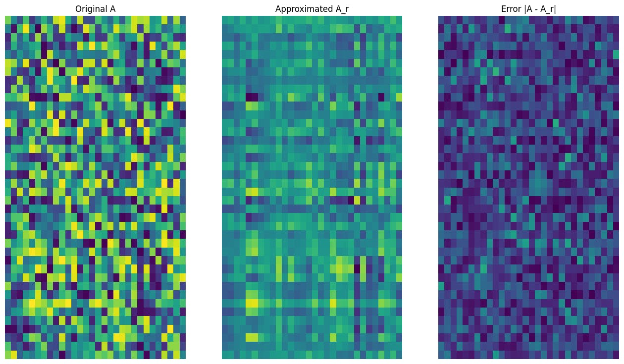
Como se esperaba, el uso de rangos más bajos da como resultado aproximaciones menos precisas. Sin embargo, la calidad de estas aproximaciones de bajo rango a menudo es lo suficientemente buena en los escenarios del mundo actual. También tenga en cuenta que el objetivo principal de la aproximación de bajo rango con SVD es reducir la dimensionalidad de los datos pero no reducir el espacio de disco de los datos en sí. Sin embargo, a medida que las matrices de entrada se vuelven de mayor dimensión, muchas aproximaciones de bajo rango también terminan beneficiándose del tamaño de datos reducido. Este beneficio de reducción es por qué el proceso es aplicable para problemas de compresión de imágenes.
Carga de imágenes
La siguiente imagen está disponible en la página de inicio de Imagen. Imagen es un modelo de difusión de texto a imagen desarrollado por el equipo cerebral de Google Analysis. Una IA creó esta imagen basada en el aviso: “Una foto de un perro Corgi montando una bicicleta en Occasions Sq.. Lleva gafas de sol y un sombrero de playa”. ¡Qué genial es eso! También puede cambiar la URL a continuación a cualquier enlace .jpg para cargar en una imagen personalizada de elección.
Comience leyendo y visualizando la imagen. Después de leer un archivo JPEG, Matplotlib emite una matriz, i, de forma (M × N × 3) que representa una imagen bidimensional con 3 canales de coloration para rojo, verde y azul respectivamente.
img_link = "
img_path = requests.get(img_link, stream=True).uncooked
I = imread(img_path, 0)
print("Enter Picture Form:", I.form)
Enter Picture Form: (1024, 1024, 3)
def show_img(I):
  # Show the picture in matplotlib
  img = plt.imshow(I)
  plt.axis('off')
  return
show_img(I)


El algoritmo de compresión de la imagen
Ahora, use el SVD para calcular las aproximaciones de bajo rango de la imagen de la muestra. Recuerde que la imagen es de forma (1024 × 1024 × 3) y que la teoría SVD solo se aplica para matrices bidimensionales. Esto significa que la imagen de la muestra debe ser un amplio en 3 matrices de tamaño igual que corresponda a cada uno de los 3 canales de coloration. Esto se puede hacer transponiendo la matriz para que tenga forma (3 × 1024 × 1024). Para visualizar claramente el error de aproximación, rescala los valores RGB de la imagen desde [0,255] a [0,1]. Recuerde recortar los valores aproximados para caer dentro de este intervalo antes de visualizarlos. El tf.clip_by_value La función es útil para esto.
def compress_image(I, r, verbose=False):
  # Compress a picture with the SVD given a rank
  I_size = tf.measurement(I)
  print(f"Unique measurement of picture: {I_size}")
  # Compute SVD of picture
  I = tf.convert_to_tensor(I)/255
  I_batched = tf.transpose(I, [2, 0, 1]) # einops.rearrange(I, 'h w c -> c h w')
  s, U, V = tf.linalg.svd(I_batched)
  # Compute low-rank approximation of picture throughout every RGB channel
  I_r, I_r_size = rank_r_approx(s, U, V, r)
  I_r = tf.transpose(I_r, [1, 2, 0]) # einops.rearrange(I_r, 'c h w -> h w c')
  I_r_prop = (I_r_size / I_size)
  if verbose:
    # Show compressed picture and attributes
    print(f"Variety of singular values utilized in compression: {r}")
    print(f"Compressed picture measurement: {I_r_size}")
    print(f"Proportion of authentic measurement: {I_r_prop:.3f}")
    ax_1 = plt.subplot(1,2,1)
    show_img(tf.clip_by_value(I_r,0.,1.))
    ax_1.set_title("Approximated picture")
    ax_2 = plt.subplot(1,2,2)
    show_img(tf.clip_by_value(0.5+abs(I-I_r),0.,1.))
    ax_2.set_title("Error")
  return I_r, I_r_prop
Ahora, calcule las aproximaciones de rango-R para los siguientes rangos: 100, 50, 10
I_100, I_100_prop = compress_image(I, 100, verbose=True)
Unique measurement of picture: 3145728
Variety of singular values utilized in compression: 100
Compressed picture measurement: 614700
Proportion of authentic measurement: 0.195


I_50, I_50_prop = compress_image(I, 50, verbose=True)
Unique measurement of picture: 3145728
Variety of singular values utilized in compression: 50
Compressed picture measurement: 307350
Proportion of authentic measurement: 0.098

I_10, I_10_prop = compress_image(I, 10, verbose=True)
Unique measurement of picture: 3145728
Variety of singular values utilized in compression: 10
Compressed picture measurement: 61470
Proportion of authentic measurement: 0.020

Evaluación de aproximaciones
Hay una variedad de métodos interesantes para medir la efectividad y tener más management sobre las aproximaciones de matriz.
Issue de compresión vs rango
Para cada una de las aproximaciones anteriores, observe cómo cambian los tamaños de datos con el rango.
plt.determine(figsize=(11,6))
plt.plot([100, 50, 10], [I_100_prop, I_50_prop, I_10_prop])
plt.xlabel("Rank")
plt.ylabel("Proportion of authentic picture measurement")
plt.title("Compression issue vs rank");


Según esta trama, existe una relación lineal entre el issue de compresión de una imagen aproximado y su rango. Para explorar esto más a fondo, recuerde que el tamaño de los datos de una matriz aproximada, AR, se outline como el número whole de elementos requeridos para su cálculo. Las siguientes ecuaciones se pueden usar para encontrar la relación entre el issue de compresión y el rango:
x = (M × R)+R+(R × N) = R × (M+N+1)
c = xy = r × (m+n+1) m × n
dónde
- x: tamaño de AR
- Y: tamaño de un
- C = xy: issue de compresión
- R: Rango de la aproximación
- my n: dimensiones de fila y columna de un
Para encontrar el rango, r, que es necesario para comprimir una imagen a un issue deseado, C, la ecuación anterior se puede reorganizar para resolver R:
R = ⌊C × M × NM+N+1⌋
Tenga en cuenta que esta fórmula es independiente de la dimensión del canal de coloration, ya que cada una de las aproximaciones RGB no se afecta entre sí. Ahora, escriba una función para comprimir una imagen de entrada dado un issue de compresión deseado.
def compress_image_with_factor(I, compression_factor, verbose=False):
  # Returns a compressed picture primarily based on a desired compression issue
  m,n,o = I.form
  r = int((compression_factor * m * n)/(m + n + 1))
  I_r, I_r_prop = compress_image(I, r, verbose=verbose)
  return I_r
Comprima una imagen al 15% de su tamaño authentic.
compression_factor = 0.15
I_r_img = compress_image_with_factor(I, compression_factor, verbose=True)
Unique measurement of picture: 3145728
Variety of singular values utilized in compression: 76
Compressed picture measurement: 467172
Proportion of authentic measurement: 0.149

Suma acumulativa de valores singulares
La suma acumulativa de los valores singulares puede ser un indicador útil para la cantidad de energía capturada por una aproximación RANCY-R. Visualice la proporción acumulativa promediada por RGB de valores singulares en la imagen de muestra. El tf.cumsum La función puede ser útil para esto.
def viz_energy(I):
  # Visualize the vitality captured primarily based on rank
  # Computing SVD
  I = tf.convert_to_tensor(I)/255
  I_batched = tf.transpose(I, [2, 0, 1])
  s, U, V = tf.linalg.svd(I_batched)
  # Plotting common proportion throughout RGB channels
  props_rgb = tf.map_fn(lambda x: tf.cumsum(x)/tf.reduce_sum(x), s)
  props_rgb_mean = tf.reduce_mean(props_rgb, axis=0)
  plt.determine(figsize=(11,6))
  plt.plot(vary(len(I)), props_rgb_mean, coloration='ok')
  plt.xlabel("Rank / singular worth quantity")
  plt.ylabel("Cumulative proportion of singular values")
  plt.title("RGB-averaged proportion of vitality captured by the primary 'r' singular values")
viz_energy(I)


Parece que más del 90% de la energía en esta imagen se captura dentro de los primeros 100 valores singulares. Ahora, escriba una función para comprimir una imagen de entrada dado un issue de retención de energía deseado.
def compress_image_with_energy(I, energy_factor, verbose=False):
  # Returns a compressed picture primarily based on a desired vitality issue
  # Computing SVD
  I_rescaled = tf.convert_to_tensor(I)/255
  I_batched = tf.transpose(I_rescaled, [2, 0, 1])
  s, U, V = tf.linalg.svd(I_batched)
  # Extracting singular values
  props_rgb = tf.map_fn(lambda x: tf.cumsum(x)/tf.reduce_sum(x), s)
  props_rgb_mean = tf.reduce_mean(props_rgb, axis=0)
  # Discover closest r that corresponds to the vitality issue
  r = tf.argmin(tf.abs(props_rgb_mean - energy_factor)) + 1
  actual_ef = props_rgb_mean[r]
  I_r, I_r_prop = compress_image(I, r, verbose=verbose)
  print(f"Proportion of vitality captured by the primary {r} singular values: {actual_ef:.3f}")
  return I_r
Comprima una imagen para retener el 75% de su energía.
energy_factor = 0.75
I_r_img = compress_image_with_energy(I, energy_factor, verbose=True)
Unique measurement of picture: 3145728
Variety of singular values utilized in compression: 35
Compressed picture measurement: 215145
Proportion of authentic measurement: 0.068
Proportion of vitality captured by the primary 35 singular values: 0.753

Error y valores singulares
También hay una relación interesante entre el error de aproximación y los valores singulares. Resulta que la norma Frobenius cuadrado de la aproximación es igual a la suma de los cuadrados de sus valores singulares que quedaron fuera:
|| A – AR || 2 = ∑i = R+1Rσi2
Pruebe esta relación con una aproximación de rango 10 de la matriz de ejemplo al comienzo de este tutorial.
s, U, V = tf.linalg.svd(A)
A_10, A_10_size = rank_r_approx(s, U, V, 10)
squared_norm = tf.norm(A - A_10)**2
s_squared_sum = tf.reduce_sum(s[10:]**2)
print(f"Squared Frobenius norm: {squared_norm:.3f}")
print(f"Sum of squared singular values omitted: {s_squared_sum:.3f}")
Squared Frobenius norm: 33.021
Sum of squared singular values omitted: 33.021
Conclusión
Este cuaderno introdujo el proceso de implementación de la descomposición del valor singular con TensorFlow y la aplicación para escribir un algoritmo de compresión de imagen. Aquí hay algunos consejos más que pueden ayudar:
Para obtener más ejemplos del uso de las API del núcleo TensorFlow, consulte la guía. Si desea obtener más información sobre la carga y la preparación de datos, consulte los tutoriales sobre la carga de datos de imágenes o la carga de datos CSV.
Publicado originalmente en el
")

")


")


